3D Bathymetry -Part 2- Kriging
Introduction.
In the first part of this article we managed to generate a sampling grid matching the contour of the surveyed area,starting from a data frame containing spatial metrics. This sampling grid will be implemented when building the krige function available with the gstat library.
Part 2 - Kriging
In a nutshell, Kriging is a geostatistical method which :
- measures spatial variability of a geographic data attribute.
- allows to predict or estimate the value at the location where the true value is unknown.
In our case, the geographic data attribute is the water depth, and the sampling grid is defining the locations where we want to predict water depth.
Another definition of kriging describes the model as a linear regression method involving combination of weights for estimating a value between sampled data, and for calculating the weighted average of known values of the neighborhood points. In other words, kriging modeling fits a mathematical function to a specified number of points, or all points within a specified perimeter, to determine the output value for each location.
Now, unlike linear regression, the assumption of independency of variables is violated in kriging. In fact we will consider that the geographic data attribute is spatially autocorrelated, meaning that there is a spatial effect on the data. Thus, kriging modeling is based on this new assumption: a cluster of points with proximity in space tend to present similar water depth characteristics.
Prior fitting the model, we will have to define a mathematical function describing the spatial dependency between two observations. Such function is called variogram. A variogram quantifies the spatial correlation and in our case will give a measure of how much two sample locations, with water depth acquired within the survey area, will vary in their water depth value depending on the distance between the two locations.
First of all, let’s set the columns X (easting) and Y (northing) of our source data frame as spatial coordinates, and set the projection.
coordinates(Source_data) <- ~ X + Y
proj4string(Source_data) <- CRS("+init=epsg:32712")
We can now calculate a sample/experimental variogram from the source data set with water depths defined as the variable response and X/Y defined as spatial coordinates.
library(gstat)
variogram <- variogram(Depth~X + Y, data =Source_data)
At sample points with close distances, the difference in values between points tend to be small. In other words, the variance is small. But when the distances between sample points are increasing, the difference in values between points are less likely to be similar. As distance increases away from sample points, there is no longer a relationship between the sample points. Their variance begins to flatten out, and sample values are not related to one another.
This can be easily checked by fitting a spherical model to the experimental variogram, plotting both the sample variogram and the variogram model fitted to it, and observing the variance:
variogram.sph.mod <- fit.variogram(variogram, vgm("Sph"))
plot(variogram,variogram.sph.mod)
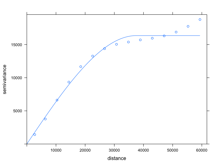
The above figure displays an experimental variogram with a variogram model fitted to it. Each blue circle is a lag of the experimental variogram, and the blue line represents the variogram model fitted. The x-axis is referring to the distance between pairs of sample points, and the y-axis represents the calculated value of the variance. A greater variance value indicates less correlation between pairs of sample points.
This particular variogram shows a spatial relationship well suited for geostatistical analysis since pairs of points are more correlated the closer they are together, and become less correlated the greater the distance between points.
The next step is to conduct ordinary kriging interpolation using krige function available with the gstat package. Ordinary kriging serves to estimate a value at a point of a region for which a variogram is known, using data in the neighborhood of the estimation location. For this purpose, various arguments will have to be implemented within krige function.
To summarize, we will have to define :
A formula that defines the dependent variable (water depth) as a linear model of independent variables. In our case we will be conducting ordinary kriging, thus using “Depth ~ 1” argument.
The data frame containing the dependent variable, and coordinates of points with acquired data.
A spatial object with prediction locations. Here we will be using the sampling grid created in Part 1 of this article, matching the exact contour of our survey area, and defined as a Spatial Pixel Data Frame object.
The variogram model fitted to our experimental variogram (variogram.sph.mod).
The number of nearest observations that should be used for the kriging prediction (in our case we will use nmax=30).
We can now start the kriging interpolation in a single command line:
Kriging_interp <- krige(Depth ~1, Source_data, newdata = Final_grid_SPDF, model=variogram.sph.mod, nmax = 30)
Let’s have a look at the result :
summary(Kriging_interp)
The result is an object of class SpatialPixelDataFrame, with two 1052205 rows corresponding to the number of water depths predictions. This amount of predicted data is expected according the dimensions of the spatial grid created during the first part of this article (920x1599). All observations cover the entire survey area and allow for a fine-grained distribution of points with predicted water depth data.
Column var1.pred in the SpatialPixelDataFrame object is referring to the predictions of water depths, and we can now plot a simple 2D map displaying the achieved kriging interpolations :
Map_2D <- spplot(Kriging_interp, "var1.pred")
print(Map_2D)
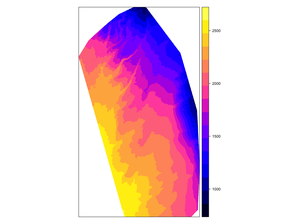
Using kriging modeling, and starting from a simple csv file, we have been able to create a 2D bathymetry map of the survey area. The next and last part of this article will discuss about 3D bathymetry map generation.
Some elements of bibliography :
For better understanding of kriging geostatistical method, it is advised to read this interesting presentation proposed by Hans Wackernagel, and go here to get directed towards the plethora of litterature on the subject.