3D Bathymetry -Part 3- Build a 3D map

Introduction.

The kriging interpolation model conducted in part 2 of this article resulted in approximately one million water depth interpolated observations covering the entire area surveyed by the vessel. We have been able to create a simple 2D bathymetry map using the output of the kriging interpolation and now we can follow a few last steps for generating a 3D bathymetry map.

Part 3 - Build a 3D map

First of all, let’s convert our SpatialPixelDataFrame object created with kriging interpolation to a data frame with 3 columns : X (easting), Y (northing), and Depths (Water depth).

As stated in part 2, water depths predictions are retrieved from the SpatialPixelDataFrame object with :

Kriging_interp$var1.pred

And X/Y projected coordinates are retrieved with :

Kriging_interp@coords

Let’s gather coordinates and water depths in a single data frame :

Kriging_interp_DF <- data.frame(Kriging_interp$var1.pred,Kriging_interp@coords)

Kriging_interp_DF
        Kriging_interp.var1.pred       s1      s2
1                       985.7814 820072.9 1515251
2                       984.3413 820172.9 1515251
3                       983.2533 820272.9 1515251
4                       982.6587 820372.9 1515251
5                       982.7211 820472.9 1515251

Some little tuning of the data frame to round water depths values, convert water depths in negative values, and rename columns :

Kriging_interp_DF$Kriging_interp.var1.pred <- round(Kriging_interp_DF$Kriging_interp.var1.pred, 0)
Kriging_interp_DF$Kriging_interp.var1.pred <- -Kriging_interp_DF$Kriging_interp.var1.pred
colnames(Kriging_interp_DF)[1] <- "Depth"
colnames(Kriging_interp_DF)[2] <- "X"
colnames(Kriging_interp_DF)[3] <- "Y"

And our data frames becomes:

Kriging_interp_DF
        Depth        X       Y
1        -986 820072.9 1515251
2        -984 820172.9 1515251
3        -983 820272.9 1515251
4        -983 820372.9 1515251
5        -983 820472.9 1515251
6        -983 820572.9 1515251

We have now a data frame containing 1052205 observations with X & Y projected coordinates and predicted water depths.

As previously mentioned, several R libraries allow for generating 3D visualization plots. Here is proposed to use the rgl library, and more specifically the "persp3d" generic function.

Persp3d, as many other 3D plot generation tool, requires a matrix as main argument, where the row index will be used for X, the column index will be used for Y, and the matrix cell values will be reflecting the Z value at cell(X,Y).

To convert our Kriging_interp_DF data frame into a matrix, we can use "acast" function available in reshape2 library.

library(reshape2)
Kriging_interp_matrix <- acast(Kriging_interp_DF, X~Y, value.var="Depth")

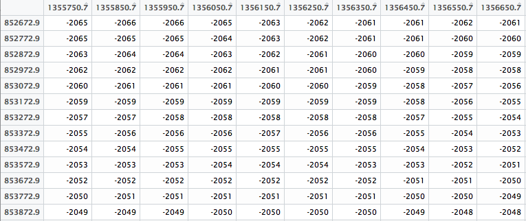
In the below screenshot of Kriging_interp_matrix, displayed using RStudio, the row index is used as X, the column index is used as Y, and the water depth are appearing in the corresponding cell. We can also note that the increment on X and Y indexes is equal to 100 meters, which is what we expect considering the definition of the 100m bin size when creating the sampling grid in part 1 of this article.

To summarize, when running persp3d, we will need to define :

• The locations of the matrix grid lines at which the values in z are measured.

• The matrix containing the values to be plotted (i.e. water depths).

• Color parameter.

• An aspect ratio.

• Any other additional parameter to be passed.

Rownames and colnames can be used to retrieve the row and column names of a matrix object. Thus, for the locations Xaxis and Yaxis of the grid lines:

Xaxis <- as.numeric(rownames(Kriging_interp_matrix))
Yaxis <- as.numeric(colnames(Kriging_interp_matrix))

Defining 100 colors of a rainbow palette (from red to blue), and breaking the water depths in 100 segments:

colors_100 <- rev(rainbow(100, start = 0/6, end = 5/6))
Depths_100_breaks  <- cut(Kriging_interp_matrix, 100)

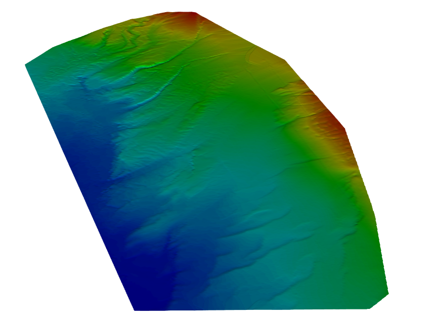
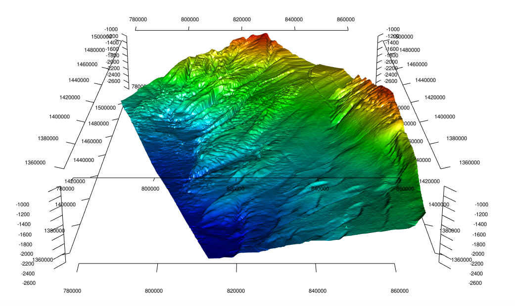
We can now generate a first 3D bathymetry map with all coordinates X, Y, and Z, at a similar scale :

persp3d(x = Xrange,
        y = Yrange,
        z = Kriging_interp_matrix,
        col = colors_100[Depths_100_breaks],
        aspect = "iso",
        xlab="", 
        ylab="", 
        axes=FALSE)

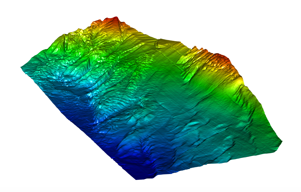
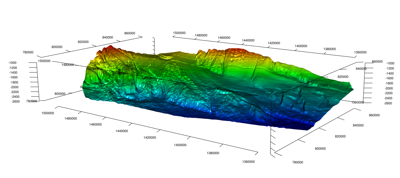
Replacing “iso” by another ratio extending Z scale provides an interesting view, although the depth variations are exaggerated:

aspect = c(4,6,1)

Adding X,Y,and Z axis:

par3d(cex = 0.7)
axis3d('z++', nticks = 10)
axis3d('z+-', nticks = 10)
axis3d('z-+', nticks = 10)
axis3d('z--', nticks = 10)
axis3d('y++', nticks = 10)
axis3d('y-+', nticks = 10)
axis3d('y+-', nticks = 10)
axis3d('y--', nticks = 10)
axis3d('x++')
axis3d('x-+')
axis3d('x+-')
axis3d('x--')

Removing the three axis and rendering as a spinning animation:

movie3d(spin3d(axis = c(0,0,1)), duration=4, dir = getwd(),  convert = TRUE)