3D Bathymetry -Part 1- Build a sampling grid

Introduction.

While conducting a marine seismic survey, a high variety of data is collected by the seismic vessel operating the survey.

In addition to the seismic data acquired, water depths measured by the vessel’s echo sounder are providing useful information about the ocean floor.

The high density of the spatial points with measured water depths makes it possible to create a 3D bathymetry map of the local area surveyed. In R, several packages allow for building 3D surface maps, such as rgl, plot3D, lattice, ...

The purpose of this article is to present a methodology for generating a 3D bathymetry map, starting from a simple csv file containing water depth data acquired at 104686 locations along 200 sail lines, with known X/Y projected coordinates. Various steps shall to be followed prior building the 3D map.

Let’s divide this article in three parts :

1. Build a sampling grid matching the survey area
2. Water depth data estimation using Kriging geostatistical method
3. Generate 3D bathymetry map
   

Part 1 - Build a sampling grid matching the survey area

Let’s start by having a look at the data :

Source_data <- read.table("Source_data.csv", header = TRUE, sep = ",")
str(Source_data)

data.frame':	104686 obs. of  5 variables:
 $ X    : num  777973 778014 778062 778118 778175 ...
 $ Y    : num  1477568 1477385 1477202 1477022 1476842 ...
 $ Long : num  95.6 95.6 95.6 95.6 95.6 ...
 $ Lat  : num  13.4 13.4 13.3 13.3 13.3 ...
 $ Depth: num  2061 2066 2069 2073 2077 ...

This data frame contains 104686 spatial points with latitude, longitude, projected X (easting) & Y (northing) coordinates, and processed echo sounder data (water depths in meters, corrected for both vessel's draft and tide).

Let’s build a simple map using X/Y coordinates from the source dataset.

library(ggplot2)
map_survey <- ggplot(data= Source_data, aes(x=X, y=Y)) 
map_survey + geom_point(colour="red",size = 0.01)

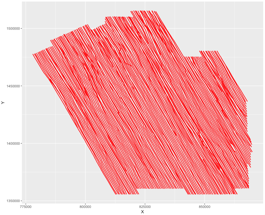
The track of the vessel can be easily observed, with sail lines having NW/SE headings. The positions of the observations appear to be quite well distributed within the survey area, covering the whole surface, but some sections of the map seem to be less covered in points than others.

Let’s zoom at the map.

map_survey + geom_point(colour="red",size = 0.05) 
           + coord_cartesian(ylim=c(1400000,1402000),xlim=c(850000,852000))

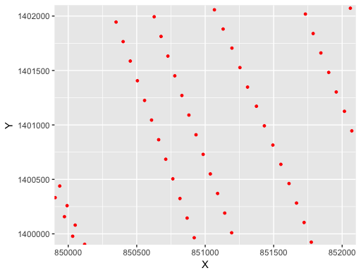
The zoomed map highlights distances between points which are obviously not equal, and the points are simply forming an irregular grid of points. However, most of the 3D mapping R functions are expecting locations of regular grid lines and a matrix object containing water depths. In other words, the main argument of a 3D mapping function must be a matrix with X rows, Y columns, and each cell containing the values of the water depths to be plotted. This matrix can be obtained by overlaying a spatial polygon with a sampling grid and interpolating water depths using kriging method.

Let’s start by creating a regular sampling grid matching the contour of the survey area.

First of all, to create a convex hull of the polygon survey using chull (library grDevices):

Survey_Contour <- chull(Source_data$X, Source_data$Y )

And the coordinates X and Y of the contour are retrieved with :

Source_data_coord_contour <- Source_data[c(Survey_Contour, Survey_Contour[1]), ] 

Keeping only X and Y coordinates :

Source_data_coord_contour <- Source_data_coord_contour[,c(1,2)]

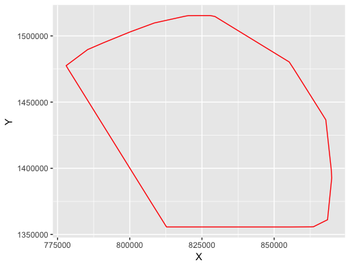
Let’s plot the contour :

map_survey <- ggplot(data=Source_data_coord_contour) 
map_survey + geom_polygon(aes(x=X, y=Y), colour="red",fill = NA) 

We now can create an object of class SpatialPolygons using sp library.

The below code is merging three steps in a single command line :

1. Step 1 - creating a Polygon object from the data frame (Survey_Contour_coord)
2. Step 2 - creating a list of Polygons objects from the Polygon object generated with step1
3. Step 3 - creating a SpatialPolygons object (Survey_Spatial_Polygon) from the list of Polygons objects generated in with step2, and specification of the desired coordinate reference system (for instance ellipsoid WGS 84, Projection UTM 12S ).

Survey_Spatial_Polygon <- SpatialPolygons(list                                            # step 3
                                          (Polygons(list                                  # step 2
                                                    (Polygon(Source_data_coord_contour)), # step 1
                                                    ID=1)),
                                          proj4string=CRS("+init=epsg:32712"))

Our SpatialPolygons object has boundary contour matching the contour of the survey area where the echo sounder data has been collected. What we need to create now is a sampling grid, defined as a regular spatial grid with a defined number of columns rows, and covering the area of study.

Let’s first define a rectangular grid with 100 meters cell size. The choice of 100m cell size is quite arbitrary. To select an appropriate cell size, one has to put two things on a balance: the accuracy of the desired depth model and the spatial density of points acquired with data. That said, the aim of this work is to produce a simple 3D map for visualization purpose, and following several tests with different cell sizes, a 100 meters cell size definition fits quite well our objective.

For the definition of the rectangular grid parameters:

min_x <- min(Source_data$X) # minimun X coordinate
min_y <- min(Source_data$Y) # minimun Y coordinate
x_length <- max(Source_data$X - min_x) # X (easting) amplitude
y_length <- max(Source_data$Y - min_y) # Y (northing) amplitude
cellsize <- 100 # height/width of cell (meter)
ncol <- round(x_length/cellsize,0) # number of columns in the grid 
nrow <- round(y_length/cellsize,0) # number of rows in the grid 

Now we can create a GridTopology object using the grid parameters specified above.

grid <- GridTopology(cellcentre.offset=c(min_x,min_y),
                     cellsize=c(cellsize,cellsize),
                     cells.dim=c(ncol,nrow))

Using the GridTopology object just created, we can now build a SpatialPixelDataFrame object covering the whole survey area, with same coordinate reference system.

grid_SPDF <- SpatialPixelsDataFrame(grid,
                                     data=data.frame(id=1:prod(ncol,nrow)),
                                     proj4string=CRS(proj4string(Survey_Spatial_Polygon)))

For checking the dimensions of our SpatialPixelsDataFrame object just created :

grid_SPDF@grid@cells.dim
>s1   s2 
 920 1599

So we have defined a rectangular grid as a SpatialPixelsDataFrame object with 920 columns and 1599 rows, covering the entire survey area, and we would like to get the SpatialPixelsDataFrame object matching the shape of the survey. To achieve this, we will have to remove the grid outside the survey area and keep only the grid inside the survey polygon. In other words we want to pass from left to right in the below figure (grid not to scale).

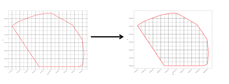
We shall then end up with an interpolation grid matching the shape of the survey area.

Let's overlay our survey polygon contour on top of the spatial grid and only select points of our grid_SPDF inside our survey polygon. This can be easily done by using over method available in sp package.

Final_grid_SPDF <- grid_SPDF[!is.na(over(grid_SPDF, Survey_Spatial_Polygon)),]

The result is a sampling grid defined as a SpatialPixelDataFrame object, matching the extend of our survey polygon. This SpatialPixelDataFrame object will be used when conducting kriging geostatistical interpolation described in the second part of this article.