Household Energy Consumption (Multilevel Model Approach) - Shiny App
Introduction.
As many other countries, France is facing the challenge of modelling its residential energy consumption (which is cccounting for more than 30% of the total energy consumption and is contributing for more than 16% of national CO2 emissions ).
Modelling residential energy consumption is essential to be able to understand national energy problematic and predict future trends, thus to be prepared to adapt policies and legislation in order to meet energy efficiency requirements at global and European levels as, for instance, the recent adopted Loi Relative à la Transition Energetique (2015)
A multilevel regression model (MRM) offers an interesting approach in the comprehension of the residential energy consumption based on the Phebus national survey” stratified dataset. MRM increases the explanatory profit when compared to classical multiple regression models that are considering only a single hierarchical level in the data. Multilevel regression models introduce simultaneously two levels of aggregation in the model, and offers the possibility of extracting contextual effects from total variation of the household energy consumption. The remaining variation is explained by the model using usual level-1 (household/individual level) explanatory variables.
Modelling approach
Most of traditional modelling approaches explaining household energy consumption in France are historically based on a single individual level model, although the dataset of reference can be considered as stratified. A few other modelling approaches, including various approaches studied in the USA, enabled to point the fact that variations of energy consumed by households can be explained not only at a individual level (household), with the inclusion of individual household’s characteristics,but also at a more aggregated level in which are considered the impact of contextual or regional effects.
The key concept here is to understand that the group in which are belonging individuals can be considered as a relevant context to the extent that it comprises a game of influences having effects on the behaviour of individuals.
Interesting approaches presented in Wang & Wang (2011) or Tso & Guan (2014) studies, indicate that area variations or regional effects have a significant impact on energy consumption. The results of both studies are showing that spatial interaction among households energy consumption in the United States becomes weaker with the farther neighbor states, thus confirming that within a same group, households can interact between themselves and may influence each other in their way of consuming energy.
Contextual Effect
Now, the questions that we would like to answer could be :
How could we quantify a contextual (or geographical) effect influencing the residential household energy consumption in France?
How much of the variation of the household energy consumption is due to the differences between the geographical divisions ?
These questions are quite relevant assuming that households leaving in different geographical divisions may differ in the way they consume energy, even if the household's characteristics are similar (income, age, type of heating system used in housing, ...). By the same reasoning, we can reasonably think that households sharing the same environment might also show some similarity in the way they are consuming energy, even if their individual characteristics are different.
The contextual effect could be due to numerous environmental indicators including cultural, economic, politic, or historic reasons. When using multilevel modeling, one is assuming that within a same group, or geographical division, individuals interact each other and therefore can mutually influence their way of consuming energy.
Phebus Dataset
Phebus National Survey is a punctual national survey conducted in France, implemented by INSEE (National Institute of Statistic and Economical Studies) and is including two sections realized separately: a face to face interview with housing occupants and a diagnosis of energy efficiency of their housing unit.
The objective of Phebus national survey is to deliver a clear photography of households energy use within French metropolitan housing stock in 2012. Phebus dataset consists of a set of metric and non-metric variables taken from 2356 housing units selected to represent the 27.6 million housing units that are occupied as a primary residence. Only housing units corresponding to an individual house, housing units located inside building, independent rooms inside buildings with private entrance, and home dedicated to elderly people are taken in consideration during data collection and survey.
Phebus survey has been conducted in 2013, across 81 “départements” (DEP) within French metropolitan territory. The survey provides detailed information regarding household characteristics aiming for better understanding of the variations of the total amount of energy yearly consumed.
Dictionary of variables
Let’s have a look on some of the data collected during the survey, and variables used for fitting our multilevel model.
Variable Response
In the model that will be conducted in this paper, the variable response is the 2012 energy consumption per household, measured in kWh. The household energy consumption corresponds to the quantity of final energy consumed by a household for space heating, production of hot water and electrical appliance in the housing.
In order to reduce the skewed distribution of the response variable, and to increase the impact of the differences between values on the left side of the distribution, where the majorities of the observations are taking place, a logarithm transformation is implemented. The transformed response variable is named LOGCONSTOT.
Level - 2 - Grouping Variables (aggregated level)
DEP is a categorical variable indicating the identification number of the “département” where is living the interviewed household. DEP consists in one of the french administrative division type.
Let’s now introduce significant level-2 predictors that may explain variation of household energy consumption. All candidate variables described below are aiming to capture regional effects on the household energy consumption.
LOGREVDEP is a numerical variable indicating the logarithm of the average per capita disposable household income, per DEP in 2012 (source of data INSEE).
HDDDEP is a numerical variable indicating the heating degree days in 2012 (source of data ADEME).
The two above level-2 explanatory variables are proposed for explaining a clustering effect within DEP geographical divisions: DEP-average per capita yearly income in 2012 (LOGREVDEP), and heating degree-day per department in 2012 (HDDDEP).
To be noted that due to homogeneous energy policies among French administrative divisions, average prices of energy remain identical across whole French territory and therefore can not be considered useful for explaining the household energy consumption in our models.
Level - 1 - Explanatory Variables (individual/housing occupants level)
LOGREV is a numerical variable indicating the gross household income disposed in 2012, with a log transformation to reduce a right skewed distribution.
AREA3G is a categorical variable indicating the area of the housing, divided in three groups: 0-40m2 ;40m2-100m2;100m2 and above.
INSULHOUS is a binary indicator measuring whether the housing is insulated (=1) or adjoining to another housing unit (=0).
YEARCONST is a numerical variable indicating the year when the house was built.
ROOMNBR is a numerical variable indicating the number of bedrooms in the housing.
HEATSYST is a categorical variable indicating whether the space heating system is dedicated only for heating the housing, for heating a cluster of housing (collective space heating system), or a mixed system (individual and collective).
HEATSOURCE indicates the type of energy used for the space heating system. Three categories are defined: electricity ; gas ; other.
RURAL is a binary indicator showing if the housing is located in a rural area (i.e. less than 2000 hab). 1= Yes, 0 = No.
HEATTEMP is another binary variable indicating the heating temperature selected by the households to heat their housing is above 21°C (included). 1= Yes, 0= No.
ECS is a categorical variable indicating how is produced hot water. Three categories are defined: Electricity, boiler (using gas, fuel, or wood as energy source), and others.
UNOCCWEEK is a binary variable indicating whether the housing is unoccupied less than four hours during weekdays. 1= Yes, 0= No.
PCS is a categorical variable indicating household employment status. Three categories are defined: Executive status, Middle-level status, and other status.
NBRPERS is a numerical variable indicating the number of persons living in housing.
Aggregation bias and various assumptions discarded
An important benefit of using multilevel models is that, by differentiating levels of analysis, it helps avoiding the aggregation bias effect (also known as the Robinson effect) which is consisting in inferring conclusions on a individual level based on data provided on an more aggregated level. Indeed, basing on results given by aggregated data models and inferring conclusions on individual behaviors (hence household energy consumption) may well turn out to be false, and lead to what can be called the aggregation bias effect. The use of multilevel regression model also helps avoiding the atomist effect which is the opposite of the aggregation effect – inferring conclusion on a aggregated level based on data provided on a single individual level.
One of the base-assumption of classical regression models is the independency of errors. This assumption is excluding a grouping effect involving that members of the same group would tend to look alike than members not belonging to the same group. Yet it is precisely the environmental and grouping effect that is studied with multilevel regression models. When using MRM, the assumption of independency of errors is discarded and replaced by intra-group (intra-class) errors, which corresponds to the fact that households within the same group, or geographical division, tend to look alike. Moreover, classical regression models are founded on the assumption of homoscedasticity of residuals, i.e. the stability of residual variance. MRM replace the homoscedasticity assumption by a weaker assumption stipulating that residual variance can vary as a linear or non-linear function of explanatory variables.
Multilevel models are mixed models adapted to stratified data analysis. It contains various error terms, at least one error term at each level of the structure model.
Fixed effects and random effects
When modeling effects of some variables, it is convenient to understand which type of effect is modelled. It is therefore important to operate a distinction between fixed effects and random effects.
Random effects are stochastic effects while fixed effects aren’t. For a good understanding of the difference between both effects, it is kindly suggested to read this stackoverflow answer.
When studying fixed effects, only effects of a specific modality of a factor on a dependent variable is assessed. With Phebus dataset, evaluating fixed effects would be limited for instance to assess the effects of the 3 housing area modalities on household energy consumption. When analyzing fixed effect, it is the precise effect of the affiliation of the household to one of the three housing area modalities that is studied.
In the present case, the goal is to understand to what extent the geographical context has a control over the household energy consumption. The geographical context can here be resumed by the level -2- grouping variables indicating where households are geographically located: DEP. It is not a particular effect of a DEP on household energy consumption that we are concerned for, but the overall effect of DEP as a grouping variable.
To summarize, fixed effects will be useful for quantifying the effect of explanatory level-1 variables (income, year of construction of the housing, type of heating system, etc..) while random effect will help us to quantify the effect of the grouping variable DEP on the household energy consumption. We do not want to know what is the effect of a specific DEP on the household energy consumption, but the effect of a DEP randomly selected from a population of DEP.
Null Model
A first step, when analyzing a stratified dataset, consists in evaluating how the variance of the studied phenomena (energy consumption) is shared among the different levels of aggregation. This can be done by fitting a null model. A null model is a multilevel model as it integrate two levels of aggregation, and is an unconditional model as no level -1- explanatory variables is introduced.
This model can be fitted with a simple line command in R, using lmer library.
NullModel <- lmer(LOGCONSTOT ~ 1 + (1 | DEP), data = Phebus)Let’s have a look at the random effect output of the null model just fitted :
Random effects:
Groups Name Variance Std.Dev.
DEP (Intercept) 0.06652 0.2579
Residual 0.52177 0.7223
Number of obs: 2090, groups: DEP, 81
This output allows us to calculate an ICC (intraclass coefficient), which corresponds to the percentage of variance between DEP compared to the global variance of the energy consumption.
An elevated ICC would indicate that the variance inter-class (in between DEP) dominate over the variance intra-class,between individual or households. In other words, that the differences observed in the household energy consumption are resulting at a great extend from the differences between the administrative divisions DEP.
We have here an ICC equal to 0.12. Thus 12% of the global variance of the consumption of energy can be attributed to the level-2- DEP. We can reasonably think that a clustering effect exists and this effect would explain 12 % of the global variance.
An effect explaining 12 % of the total variance is not spectacular, but also is not negligible, and we can try to minimize the 88% of the residual variance, non explained by the null model, by introducing level -1- and level -2- explanatory variables in a multilevel model.
Multilevel Model
A random-intercept multilevel model can be transposed with the following equation:
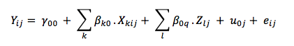
Where:
𝑌ij is the annual energy consumption of household i in geographical division j (DEP).
𝑋ij is the matrix of level-1 explanatory variables.
𝑍j is the matrix of level-2 explanatory variables.
Other parameters in the equation need to be estimated.
For fixed effects, 𝛾00 is the intercept for fixed effects, 𝛽k0 is the slope for level-1 explanatory variables, and 𝛽0q is the slope for level-2 explanatory variables.
For random effects, 𝑒ij is the residual term at level-1 (households) and 𝑢0j is the residual term at level-2 (DEP). The variance of the residual error 𝑢0j is the variance of the intercepts between DEPs.
This model can be fitted with a simple line command in R :
Multilevel_Model <- lmer(LOGCONSTOT ~ 1 + LOGHDDDEP + LOGREVDEP + LOGREV + AREA3G + INSULHOUS +
YEARCONST + ROOMNBR + HEATSYST + HEATSOURCE + RURAL +
HEATTEMP + ECS + UNOCCWEEK + PCS + NBRPERS +
(1 | DEP), data= phebus, REML =FALSE)
It is reminded here that the above model is a random-intercept type, hence it considers that there is a different intercept for each DEP. In fact we will consider that the year of construction of a housing or the income of the household does not have the same effect on the energy consumption whether the household lives in Paris or in Gironde, or in any other DEP.
In multilevel models, there are as many variances as levels incorporated in the model. For appreciating the relevance of a multilevel model compared to another, it is suggested to observe the variance of the random effects in each level, and make the comparison to the variance obtained with the null model. In other words, the null model will act as a reference model, and we will quantify the reduction of the residual variance.
The below table summarizes the random effects output for both null model and our multilevel model we just fit.
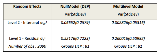
The evolution of the estimations of the random effects between both models is quite interesting. Passing from a null model to a multilevel brought an explanatory profit. Let’s examine this explanatory profit level by level. At level-1 (households), residual variance is 0.52176 for Null model and is 0.260016 for the multilevel model. Thus, the explanatory profit of the multilevel model is (0.52176-0.260016)/0.52176 = 0.502.
We can assume that the multilevel model highlights a contextual effect corresponding to 12 % of the global variance of the household energy consumption, and that 50 % of the residual variance is explained by explanatory variables at level -1- and level -2-.
Conclusion
Scientists are usually describing a society with a hierarchical structure. Multilevel models were developed to appropriately represent such data structures by incorporating hierarchical levels inside the model. Most of residential energy consumption models created in the past, and based on datasets provided from various surveys, were built under standard multiple regression frameworks with usual variables taken in account for explaining the residential energy consumption. Those standard models are generally not capable of capturing more than 55% of the residential energy consumption variance.
Modeling the household energy consumption using a multilevel model allows for better understanding and increases the explanatory profit when compared to classical multiple regression models that are considering only a single hierarchical level in the data. This article tends to suggest that, while individual or level-1 information explains a larger part of energy consumption variation (88 % of global variance), there is some statistical evidence for contextual effects in the household energy consumption variation within French departments (12% of global variance).
However, Multilevel regression modeling also has its limitations. Firstly our sample size taken from Phebus dataset might un-sufficiently large to draw inference for a population of households and departments. Secondly, the results of the ad hoc geographical clustering confirmed the significant regional effect on households energy consumption, but the interpretation of the results was proved to be quite complex. In effect, although a multilevel model is increasing the explanatory profit from 55% to 67% of the global variance of the household energy consumption, it is quite difficult to precisely analyze and quantify the geographical effect of one specific department compared to another. To improve the model, another forward step would be to study a random slope and intercept model, or studying interaction between variables in the same model, which would have as well brought more complexity in the interpretation of the results of such model.
Shiny App - Predictive Multilevel Model
Our Multilevel Model described above has been implemented in a Shiny App for building a predictive model. Playing interactively with some level-1 predictors, one can easily predict the household yearly energy consumption in each geographical division DEP, according the value chosen selected for each one of the predictors. Level-2- residuals calculated with the multilevel model, as well as several other indicators are available in the tab “Descriptive - Map of indicators. The full dataset is visible in tab “Phebus Data Table”.
The below map is indicating what would be the household yearly energy consumption on each geographical division department (DEP) if the household has a yearly income of 30k€, living a housing surface comprised between 40 and 100m2, in a insulated housing (not attached to other housing) built before 1975, with 3 rooms, an individual heating system, etc…
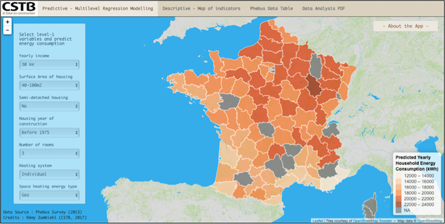
Full code of the Shiny App available here.